Welcome to the second post from my collaboration with @chrismattman. We were both intrigued when Google announced a significant upgrade to their search algorithm in late 2019. The technique is super cool, inspired by the human brain, redefining how we search for text, images, music, and more.
Here’s one example from Google’s post. Let’s say we’re wondering whether we can pick up medicine for a friend, who may be sick and cannot enter a pharmacy due to Covid19 restrictions. We Google it:

Before this upgrade, Google would show us information about prescriptions on the left. Old Google would see high overlap between our keywords “get, pharmacy, medicine” and the top blog post. Statistically, these keywords are the meaty, distinguishing topic of our inquiry. The rest of the words are quite common, such as “can, you,” and “for”. Articles that only include those wouldn’t do us much good. Google would seek keyword overlap, finding the most authoritative and relevant answer. This is how search has worked for decades, which we call syntactic search, based on the written syntax of human language.
The new Google thinks differently. The new Google thinks like Bert with tensors, as described in our previous blog post. Here Google understands that “can, for, someone” are key to our intent, even though the common words of “for” and “someone” seem to carry little information by themselves. These words, along with the major keywords of “get, pharmacy, medicine” better define our intent, encoded as a tensor. Sure enough, today’s new Google finds a better article on the right. Note that the article talks of “prescription” when we stated “medicine,” though these are clearly related, even though they don’t match. This new approach is called semantic search and it’s here and widely available and easily implemented because of Bert.
Semantic search is cool. It’s all the rage in the scientific community. We have high hopes that this tensor technique will allow us to better search through our overfull inboxes, that pile of PDFs waiting to be read, or the thousands of customer comments we’d like to process.
How it Works
Semantic search is a three-step process.
- Encode content as tensors
- Encode a query as a tensor
- Find tensors that match
Encoding content
We need a tool for turning content into tensors in bulk. Currently this remains the realm of research, though we suspect this capability will soon be commercially available. Please, are you listening, product people? Bueller? Has anyone seen Bueller?
We have two current favorites, one for scale, one for play.
Bert as a Service, for scale.
Han Xiao (@hxiao) released an open source package in 2019 which takes the latest, published version of Bert and encapsulates it in a web service. Han was recently a CTO at TenCent, now building a promising new company (Jina.ai) for semantic search.
Han applied hardcore, distributed systems engineering and optimizations which allows us to turn 256 sentence fragments into embeddings with a single call, automatically and elegantly handled by a powerful cluster of energy-chomping, GPU-enhanced, computational beasts. We extended his code to run Bert on Google Cloud in a public Github repository; feel free to use it!
We use Bert as a Service in our applied AI work at Google and NASA, as it scales
nicely to handle millions of sentences. If you’ve ever written a function in
Microsoft Excel, say, for taking the @sum() of a column, you now have what it
takes to use Bert!
Thanks to Bert as a Service, here’s how we turn three sentences about “apples” into tensors:
apple1 = bertify("Apple shares rose on the news.")
apple2 = bertify("Apple sold fewer iPhones this quarter.")
apple3 = bertify("Apple pie is delicious.")
The values “apple1, apple2,” and “apple3” are 768-dimensional vectors representing the BERT tensors. We can execute these in parallel too, up to 256 at a time. These are sent to a cloud service that can use your own, private cluster of high-end, GPU-stuffed machines:
apples = bertify(["Apple shares rose on the news.",
                "Apple sold fewer iPhones this quarter.",
                 "Apple pie is delicious."])
Spacy, for play.
Ines Montani (@_inesmontani) and her co-founder started explosion.ai in 2016 to make tools for processing human language. This kick-ass AI leader and her tiny German company are having an outsized impact by focusing on simple, easy to use tools that have immediate, practical value. They contribute some of their best work to open source, as part of the “spaCy” toolset.
Spacy provides tools for running Bert on your own, personal machine. With 2-3 lines of code, you can be up and running:
!pip -q install -U spacy download spacy-transformers
!pip -q install -U en_trf_bertbaseuncased_lg

import spacy
import en_trf_bertbaseuncased_lg

nlp = en_trf_bertbaseuncased_lg.load()
apple1 = nlp("Apple shares rose on the news.")
apple2 = nlp("Apple sold fewer iPhones this quarter.")
apple3 = nlp("Apple pie is delicious.")
The values “apple1, apple2,” and “apple3” are objects where you can directly access their BERT .tensor values. We find this helpful in our personal and exploratory research, where encoding a few thousand sentences is sufficient. Again, it’s no more difficult than a one-line script in Excel!
We realize there are numerous other packages and research papers on how to use Bert and its derivatives. We like things simple and believe that’s the way forward for mere mortals and also for your favorite blog authors trying to get out a blog every few weeks. If you’re not mentioned here, it’s because we find it too hard to use or, frankly, are naively unaware. Please keep pushing and sharing! The world needs your contributions to make AI simpler for all.
Our projects use these one-line interfaces to turn large quantities of raw text into large quantities of tensors. For now, we store these tensors and their original text in cloud databases such as BigQuery or cloud storage such as GCS. Absent those excellent databases, Pandas also works fine locally.
What we really want is a tensor store, optimized for storing, searching and retrieving billions of high-dimensional tensors. Feature stores are a step in the right direction, though they’re optimized for smaller vector sizes from hand-built statistical features. True tensor stores don’t yet exist.
Encoding query
The simplest approach encodes our query with a single call, as shown above. This yields a single, 768-dimensional tensor to represent our search phrase.
In Spacy,
query = nlp("Can you get medicine for someone pharmacy")
In Bert as a Service,
query = bertify("Can you get medicine for someone pharmacy")
Sophisticated, production systems like Google extend our initial query with similar words to account for mis-spellings, synonyms, and omissions. This produces not one but a set of tensors to represent our search. One shot becomes buckshot. Throw more at the wall and see what sticks. Yes, even AI uses techniques from the era of cave dwellers and knuckle draggers.
Finding tensors that match
Remember the neural science that inspired Bert? We humans encode language in the brain’s neocortex, a three-dimensional space. MRI scans revealed that similar language terms (such as “medical” and “pharmacy”) often land on the same 3D spots of the brain. Thus, when we ask you for the first word that comes to mind in a matching game, chances are you’re using the same part of your brain!
Tensors encode language in a space, too. Computers aren’t limited to 3D; the Bert algorithm reasons in a 768-D space. Similar concepts are stored close together, much like the neocortex. We want our search engine to show us the exact match, if it exists, followed by closely related text.
Here’s a plot taken from Bert answering a query, simplified to 3D. Our query’s the pale blue dot. The closest tensors in the tensor universe are displayed in colors, varying in intensity based on distance to our blue query. This is how Bert searches, as well as how NASA searches for exoplanets and extraterrestrial life (true story!).
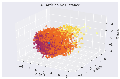
Computer scientists call this the nearest neighbor problem.
Given an input tensor T0, find the k nearest, neighboring tensors from a larger set of tensors T. T0 is blue in the figure above, along with the 1000 closest tensors (k=1000). “Nearest” is defined as the shortest line you could draw – in 768D – from one tensor to another. There’s a bit of math involved to calculate this distance, often taking a dozen instructions on a modern computer. That normally wouldn’t be bad, except for scale and impatience.
The set T of tensors is often massive, on the order of billions of tensors for a typical enterprise, trillions for the Internet. Imagine encoding all social media posts, or all documents in your enterprise, all email words and sentences. Please stay away from Chris’s posts because that’s scale. We mean nearly 43K posts of scale:

Impatience is about the speed of business. We’re accustomed to Google searches returning in under a second, from billions of web pages. We expect and want the same from semantic search. This is impatience.
Comparing the distance from our query to every tensor could take minutes on modern distributed computers. This ensures perfect recall but seemingly takes forever in a world expecting instant results.
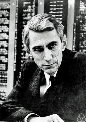
You’re probably scowling right now, as Claude Shannon was in this cropped photo from Wikipedia. Claude was the father of modern information theory which became the mathematical backbone to cracking cryptographic codes in World Wars, to building the first computers, to deploying the first cell phones, and more recently to developing the first vaccines for Covid19.
Claude formalized the idea of a “bit” of information, the smallest glimmer of information we can understand from any source. These bits were encoded as 1’s and 0’s in modern computers. Claude’s work inspired a clever solution to the nearest neighbor problem.
Let’s focus on the information in a tensor.
A tensor’s captured by modern computers as a string of bits, of 1’s and 0’s. That string of 1’s and 0’s forms a unique pattern representing the 768 different floating point numbers in a Bert tensor. We can think of the nearest neighbor algorithm as seeking tensors which represent similar, if not identical information.

In a modern computer, all our fancy nearest-neighbor math reduces to finding patterns of 1’s and 0’s that are similar to one another. What if we started there, instead, at the bit level and ignored the higher level math?
In that case, we’d be looking for patterns of 1’s and 0’s which are similar. This is how our visual system functions when staring at pictures on a computer screen. Our eyes observe millions of pixels, our brain identifies a broad pattern, calling out “cat” or “dog” as appropriate.
What we want is to find a set of tensors where their bit patterns only vary by a few, individual bits. An exact match would have no variance. Claude and his friends call this the Hamming Distance between two bit vectors.
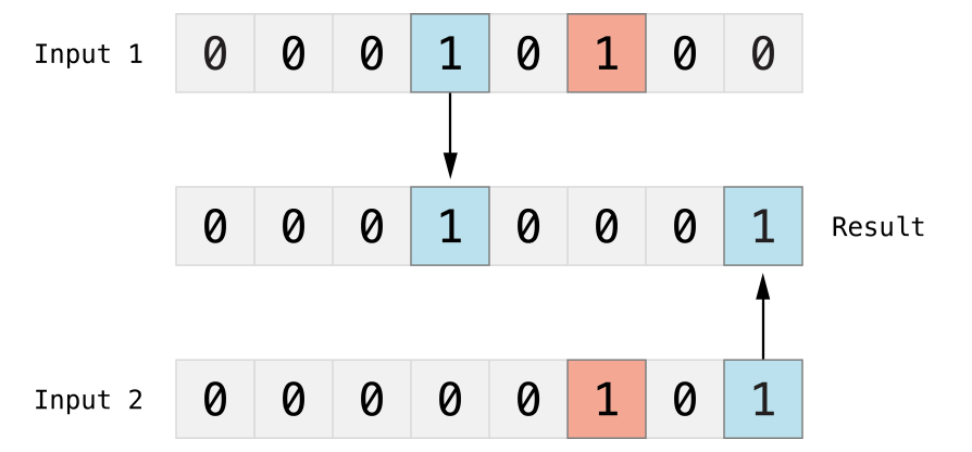
The diagram below shows the critical trick to performing nearest neighbor at scale. We take two input tensors, then XOR them. The “XOR” result returns 1 when bits differ (in blue), 0 when bits are the same (in red). We seek a result with the least number of 1’s.
That’s right. We XOR tensors, then count the 1’s. The fewer the 1’s, the closer we are. That’s it! Doing this at scale requires some clever engineering and math, but that’s the basic hack.
Intel released special computer instructions in 2013 that allow us to calculate part of the hamming distance between two tensors in a single clock cycle. The latest chips perform over 1.3 billion clock cycles per second. The latest, optimized algorithms use these instructions to process nearly a billion comparisons per second on a single computer chip. Google has millions of these chips. Now that’s some serious horsepower!
The astute reader will note that this isn’t the same as computing the shortest line between two points. That’s certainly true for low dimensional spaces, like the 3D world in which we live. I could change a single bit and scale one dimension by ten million fold! That’s hardly a match, having one dimension off by a factor of ten million.
A funny thing happens in math as we scale dimensions. As dimensions increase, they seem to fold in on each other. With one thousand dimensions, an error of ten million on one dimension could be taken as “noise,” especially when the rest of the vector lines up perfectly.
For example, if I show you a car in sunlight and a part of it reflects the sun into your eye, that small part will feel incredibly intense, causing you to squint. That intensity may be tens of thousands of times more intense than all other input, yet you still recognize the item… as a car. We discount anomalies when seeking a general pattern.
[ed. As an aside, production systems realize that Shannon’s approach is an approximation. Most production systems double check results by using higher level mathematics. Interestingly enough, the set of results from Shannon’s approach is good enough for most business needs! Researchers continue to push the frontier here, in search of even better, hybrid approaches.]
How can you access this power? Google Cloud is releasing Google’s massive capability as a new, nearest neighbor search API in 2020. Contact @scottpenberthy to get on the early access list. You can also use Facebook AI’s Similarity Search (FAISS) which is perfect for exploring and learning, or perhaps building your own service.
In both systems, we first upload our tensors then ask the system to “train,” where it creates internal data structures and maps tensors to the Hamming distance optimizations described here. Once this is done, retrieval is nearly instantaneous with a single function call:
>>> nearest("Can you get medicine for someone pharmacy")
[“https://www.hhs.gov/hipaa/for-professionals/faq/263/can-a-patient-have-a-friend-or-family-member-pick-up-a-prescription/index.html”]
Thanks to Claude Shannon, Intel, NVidia and some ingenious engineers at Google, Facebook and elsewhere, we have nearly instant retrieval at our fingertips. As before, we can reduce this ingenuity to a simple one-line function as we’ve seen in Excel.
Tensor search with scalable, nearest neighbors will be critical for all AI systems in the future, as we encode images, music, video, speech, text and more. In fact, it’s overtaking the systems behind search, online video and social feeds as we speak!
Get Started Now
We have created a free Jupyter notebook for you to play with Bert’s semantic search capabilities today. The notebook shows the three steps of semantic search:
-
We download the free, open source King James bible and encode all verses, from all 66 books, as individual tensors. We store the bible chapters, verses and tensors on BigQuery.
-
We encode our query “ask and ye shall receive” as a tensor.
-
We load all Bible verse tensors into FAISS, ask the algorithm to “train,” then send in our query. Then we pray for good results. What do you think? You be the judge. Remember, only the penitent man shall pass. Heck, with Bert, you’ll be as quick as Indy on his way to the Grail like below.

Ask and Ye Shall Receive
>>> nearest('ask and ye shall receive')

Luke 11:9 And I say unto you, Ask, and it shall be given you; seek, and ye shall
find; knock, and it shall be opened unto you.

Matthew 7:7 Ask, and it shall be given you; seek, and ye shall find; knock, and
it shall be opened unto you:

Job 33:33 If not, hearken unto me: hold thy peace, and I shall teach thee
wisdom.

Jeremiah 29:12 Then shall ye call upon me, and ye shall go and pray unto me, and
I will hearken unto you.